Bedtools Tutorial

• Table of Contents

• Synopsis
• Setup
• What are these files?
• The bedtools help
• bedtools “intersect”
  • Default behavior
  • Reporting the original feature in each file.
  • How many base pairs of overlap were there?
  • Counting the number of overlapping features.
  • Find features that DO NOT overlap
  • Require a minimal fraction of overlap.
  • Faster analysis via sorted data.
  • Intersecting multiple files at once.
• bedtools “merge”
  • Input must be sorted
  • Merge intervals.
  • Count the number of overlapping intervals.
  • Merging features that are close to one another.
  • Listing the name of each of the exons that were merged.
• bedtools “complement”
• bedtools “genomecov”
  • Producing BEDGRAPH output
• Sophistication through chaining multiple bedtools
• Principal component analysis
  • A Jaccard statistic for all 400 pairwise comparisons.
• Puzzles to help teach you more bedtools.

Synopsis

Our goal is to work through examples that demonstrate how to explore, process and manipulate genomic interval files (e.g., BED, VCF, BAM) with the bedtools software package.

Some of our analysis will be based upon the Maurano et al exploration of DnaseI hypersensitivity sites in hundreds of primary tissue types.

Maurano et al. Systematic Localization of Common Disease-Associated Variation in Regulatory DNA. Science. 2012. Vol. 337 no. 6099 pp. 1190-1195.

www.sciencemag.org/content/337/6099/1190.short

This tutorial is merely meant as an introduction to whet your appetite. There are many, many more tools and options than presented here. We therefore encourage you to read the bedtools documentation.

NOTE: We recommend making your browser window as large as possible because some of the examples yield “wide” results and more screen real estate will help make the results clearer.-

Setup

From the Terminal, create a new directory on your Desktop called bedtools-demo (it doesn’t really matter where you create this directory).

cd ~/Desktop
mkdir bedtools-demo

Navigate into that directory.

cd bedtools-demo

Download the sample BED files I have provided.

curl -O https://bedtools-tutorials.s3.amazonaws.com/curr-proc-bx/maurano.dnaseI.tgz
curl -O https://bedtools-tutorials.s3.amazonaws.com/curr-proc-bx/cpg.bed
curl -O https://bedtools-tutorials.s3.amazonaws.com/curr-proc-bx/exons.bed
curl -O https://bedtools-tutorials.s3.amazonaws.com/curr-proc-bx/gwas.bed
curl -O https://bedtools-tutorials.s3.amazonaws.com/curr-proc-bx/genome.txt
curl -O https://bedtools-tutorials.s3.amazonaws.com/curr-proc-bx/hesc.chromHmm.bed

Now, we need to extract all of the 20 Dnase I hypersensitivity BED files from the “tarball” named maurano.dnaseI.tgz.

tar -zxvf maurano.dnaseI.tgz
rm maurano.dnaseI.tgz

Let’s take a look at what files we now have.

ls -1

What are these files?

Your directory should now contain 23 BED files and 1 genome file. Twenty of these files (those starting with “f” for “fetal tissue”) reflect Dnase I hypersensitivity sites measured in twenty different fetal tissue samples from the brain, heart, intestine, kidney, lung, muscle, skin, and stomach.

In addition: cpg.bed represents CpG islands in the human genome; exons.bed represents RefSeq exons from human genes; gwas.bed represents human disease-associated SNPs that were identified in genome-wide association studies (GWAS); hesc.chromHmm.bed represents the predicted function (by chromHMM) of each interval in the genome of a human embryonic stem cell based upon ChIP-seq experiments from ENCODE.

The latter 4 files were extracted from the UCSC Genome Browser’s Table Browser.

In order to have a rough sense of the data, let’s load the cpg.bed, exons.bed, gwas.bed, and hesc.chromHmm.bed files into IGV. To do this, launch IGV, then click File->Load from File. Then select the four files. IGV will warn you that you need to create an index for a couple of the files. Just click OK, as these indices are created automatically and speed up the processing for IGV.

Once loaded, navigate to TP53 by typing TP53 in the search bar. Change the track height to 200 for each track, set the font size to 16 for each track, and change the track colors to match the following image:

Visualization in IGV or other browsers such as UCSC is a tremendously useful way to make sure that your results make sense to your eye. Coveniently, a subset of bedtools is built-into IGV!

The bedtools help

Bedtools is a command-line tool. To bring up the help, just type

bedtools

As you can see, there are multiple “subcommands” and for bedtools to work you must tell it which subcommand you want to use. Examples:

bedtools intersect
bedtools merge
bedtools subtract

What version am I using?

bedtools --version

How can I get more help?

bedtools --contact

bedtools “intersect”

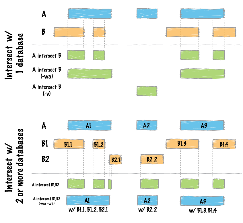
The intersect command is the workhorse of the bedtools suite. It compares two or more BED/BAM/VCF/GFF files and identifies all the regions in the gemome where the features in the two files overlap (that is, share at least one base pair in common).

Default behavior

By default, intersect reports the intervals that represent overlaps between your two files. To demonstrate, let’s identify all of the CpG islands that overlap exons.

bedtools intersect -a cpg.bed -b exons.bed | head -5
chr1    29320   29370   CpG:_116
chr1    135124  135563  CpG:_30
chr1    327790  328229  CpG:_29
chr1    327790  328229  CpG:_29
chr1    327790  328229  CpG:_29

NOTE: In this case, the intervals reported are NOT the original CpG intervals, but rather a refined interval reflecting solely the portion of each original CpG interval that overlapped with the exon(s).

Reporting the original feature in each file.

The -wa (write A) and -wb (write B) options allow one to see the original records from the A and B files that overlapped. As such, instead of not only showing you where the intersections occurred, it shows you what intersected.

bedtools intersect -a cpg.bed -b exons.bed -wa -wb \
| head -5
chr1    28735   29810   CpG:_116    chr1    29320   29370   NR_024540_exon_10_0_chr1_29321_r        -
chr1    135124  135563  CpG:_30 chr1    134772  139696  NR_039983_exon_0_0_chr1_134773_r    0   -
chr1    327790  328229  CpG:_29 chr1    324438  328581  NR_028322_exon_2_0_chr1_324439_f    0   +
chr1    327790  328229  CpG:_29 chr1    324438  328581  NR_028325_exon_2_0_chr1_324439_f    0   +
chr1    327790  328229  CpG:_29 chr1    327035  328581  NR_028327_exon_3_0_chr1_327036_f    0   +

How many base pairs of overlap were there?

The -wo (write overlap) option allows one to also report the number of base pairs of overlap between the features that overlap between each of the files.

bedtools intersect -a cpg.bed -b exons.bed -wo \
| head -10
chr1    28735   29810   CpG:_116    chr1    29320   29370   NR_024540_exon_10_0_chr1_29321_r        -   50
chr1    135124  135563  CpG:_30 chr1    134772  139696  NR_039983_exon_0_0_chr1_134773_r    0       439
chr1    327790  328229  CpG:_29 chr1    324438  328581  NR_028322_exon_2_0_chr1_324439_f    0       439
chr1    327790  328229  CpG:_29 chr1    324438  328581  NR_028325_exon_2_0_chr1_324439_f    0       439
chr1    327790  328229  CpG:_29 chr1    327035  328581  NR_028327_exon_3_0_chr1_327036_f    0       439
chr1    713984  714547  CpG:_60 chr1    713663  714068  NR_033908_exon_6_0_chr1_713664_r    0       84
chr1    762416  763445  CpG:_115    chr1    761585  762902  NR_024321_exon_0_0_chr1_761586_r        -   486
chr1    762416  763445  CpG:_115    chr1    762970  763155  NR_015368_exon_0_0_chr1_762971_f        +   185
chr1    762416  763445  CpG:_115    chr1    762970  763155  NR_047519_exon_0_0_chr1_762971_f        +   185
chr1    762416  763445  CpG:_115    chr1    762970  763155  NR_047520_exon_0_0_chr1_762971_f        +   185

Counting the number of overlapping features.

We can also count, for each feature in the “A” file, the number of overlapping features in the “B” file. This is handled with the -c option.

bedtools intersect -a cpg.bed -b exons.bed -c \
| head
chr1    28735   29810   CpG:_116    1
chr1    135124  135563  CpG:_30 1
chr1    327790  328229  CpG:_29 3
chr1    437151  438164  CpG:_84 0
chr1    449273  450544  CpG:_99 0
chr1    533219  534114  CpG:_94 0
chr1    544738  546649  CpG:_171    0
chr1    713984  714547  CpG:_60 1
chr1    762416  763445  CpG:_115    10
chr1    788863  789211  CpG:_28 9

Find features that DO NOT overlap

Often we want to identify those features in our A file that do not overlap features in the B file. The -v option is your friend in this case.

bedtools intersect -a cpg.bed -b exons.bed -v \
| head
chr1    437151  438164  CpG:_84
chr1    449273  450544  CpG:_99
chr1    533219  534114  CpG:_94
chr1    544738  546649  CpG:_171
chr1    801975  802338  CpG:_24
chr1    805198  805628  CpG:_50
chr1    839694  840619  CpG:_83
chr1    844299  845883  CpG:_153
chr1    912869  913153  CpG:_28
chr1    919726  919927  CpG:_15

Require a minimal fraction of overlap.

Recall that the default is to report overlaps between features in A and B so long as at least one basepair of overlap exists. However, the -f option allows you to specify what fraction of each feature in A should be overlapped by a feature in B before it is reported.

Let’s be more strict and require 50% of overlap.

bedtools intersect -a cpg.bed -b exons.bed \
-wo -f 0.50 \
| head
chr1    135124  135563  CpG:_30 chr1    134772  139696  NR_039983_exon_0_0_chr1_134773_r    0       439
chr1    327790  328229  CpG:_29 chr1    324438  328581  NR_028322_exon_2_0_chr1_324439_f    0       439
chr1    327790  328229  CpG:_29 chr1    324438  328581  NR_028325_exon_2_0_chr1_324439_f    0       439
chr1    327790  328229  CpG:_29 chr1    327035  328581  NR_028327_exon_3_0_chr1_327036_f    0       439
chr1    788863  789211  CpG:_28 chr1    788770  794826  NR_047519_exon_5_0_chr1_788771_f    0       348
chr1    788863  789211  CpG:_28 chr1    788770  794826  NR_047521_exon_4_0_chr1_788771_f    0       348
chr1    788863  789211  CpG:_28 chr1    788770  794826  NR_047523_exon_3_0_chr1_788771_f    0       348
chr1    788863  789211  CpG:_28 chr1    788770  794826  NR_047524_exon_3_0_chr1_788771_f    0       348
chr1    788863  789211  CpG:_28 chr1    788770  794826  NR_047525_exon_4_0_chr1_788771_f    0       348
chr1    788863  789211  CpG:_28 chr1    788858  794826  NR_047520_exon_6_0_chr1_788859_f    0       348

Faster analysis via sorted data.

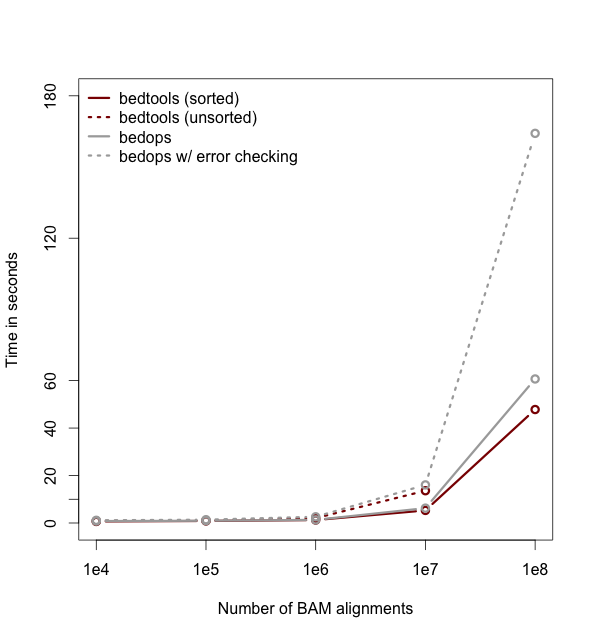
So far the examples presented have used the traditional algorithm in bedtools for finding intersections. It turns out, however, that bedtools is much faster when using presorted data.

For example, compare the difference in speed between the two approaches when finding intersections between exons.bed and hesc.chromHmm.bed:

time bedtools intersect -a gwas.bed -b hesc.chromHmm.bed > /dev/null
1.10s user 0.11s system 99% cpu 1.206 total

time bedtools intersect -a gwas.bed -b hesc.chromHmm.bed -sorted > /dev/null
0.36s user 0.01s system 99% cpu 0.368 total

NOTE: While the run times in this example are quite small, the performance gains from using the -sorted option groqw as datasets grow larger. For example, compare the runtimes of the sorted and unsorted approaches as a function of dataset size in the figure below. The important thing to remember is that each dataset must be sorted by chromosome and then by start position: sort -k1,1 -k2,2n.-

Intersecting multiple files at once.

As of version 2.21.0, bedtools is able to intersect an “A” file against one or more “B” files. This greatly simplifies analyses involving multiple datasets relevant to a given experiment. For example, let’s intersect exons with CpG islands, GWAS SNPs, an the ChromHMM annotations.

bedtools intersect -a exons.bed -b cpg.bed gwas.bed hesc.chromHmm.bed -sorted | head
chr1    11873   11937   NR_046018_exon_0_0_chr1_11874_f 0   +
chr1    11937   12137   NR_046018_exon_0_0_chr1_11874_f 0   +
chr1    12137   12227   NR_046018_exon_0_0_chr1_11874_f 0   +
chr1    12612   12721   NR_046018_exon_1_0_chr1_12613_f 0   +
chr1    13220   14137   NR_046018_exon_2_0_chr1_13221_f 0   +
chr1    14137   14409   NR_046018_exon_2_0_chr1_13221_f 0   +
chr1    14361   14829   NR_024540_exon_0_0_chr1_14362_r 0   -
chr1    14969   15038   NR_024540_exon_1_0_chr1_14970_r 0   -
chr1    15795   15947   NR_024540_exon_2_0_chr1_15796_r 0   -
chr1    16606   16765   NR_024540_exon_3_0_chr1_16607_r 0   -

Now by default, this isn’t incredibly informative as we can’t tell which of the three “B” files yielded the intersection with each exon. However, if we use the -wa and wb options, we can see from which file number (following the order of the files given on the command line) the intersection came. In this case, the 7th column reflects this file number.

bedtools intersect -a exons.bed -b cpg.bed gwas.bed hesc.chromHmm.bed -sorted -wa -wb \
  | head -10000 \
  | tail -10
chr1    27632676    27635124    NM_001276252_exon_15_0_chr1_27632677_f  0   +   3   chr1    27633213    27635013    5_Strong_Enhancer
chr1    27632676    27635124    NM_001276252_exon_15_0_chr1_27632677_f  0   +   3   chr1    27635013    27635413    7_Weak_Enhancer
chr1    27632676    27635124    NM_015023_exon_15_0_chr1_27632677_f 0   +   3   chr1    27632613    27632813    6_Weak_Enhancer
chr1    27632676    27635124    NM_015023_exon_15_0_chr1_27632677_f 0   +   3   chr1    27632813    27633213    7_Weak_Enhancer
chr1    27632676    27635124    NM_015023_exon_15_0_chr1_27632677_f 0   +   3   chr1    27633213    27635013    5_Strong_Enhancer
chr1    27632676    27635124    NM_015023_exon_15_0_chr1_27632677_f 0   +   3   chr1    27635013    27635413    7_Weak_Enhancer
chr1    27648635    27648882    NM_032125_exon_0_0_chr1_27648636_f  0   +   1   chr1    27648453    27649006    CpG:_63
chr1    27648635    27648882    NM_032125_exon_0_0_chr1_27648636_f  0   +   3   chr1    27648613    27649413    1_Active_Promoter
chr1    27648635    27648882    NR_037576_exon_0_0_chr1_27648636_f  0   +   1   chr1    27648453    27649006    CpG:_63
chr1    27648635    27648882    NR_037576_exon_0_0_chr1_27648636_f  0   +   3   chr1    27648613    27649413    1_Active_Promoter

Additionally, one can use file “labels” instead of file numbers to facilitate interpretation, especially when there are many files involved.

bedtools intersect -a exons.bed -b cpg.bed gwas.bed hesc.chromHmm.bed -sorted -wa -wb -names cpg gwas chromhmm \
  | head -10000 \
  | tail -10
chr1    27632676    27635124    NM_001276252_exon_15_0_chr1_27632677_f  0   +   chromhmm    chr1    27633213    27635013    5_Strong_Enhancer
chr1    27632676    27635124    NM_001276252_exon_15_0_chr1_27632677_f  0   +   chromhmm    chr1    27635013    27635413    7_Weak_Enhancer
chr1    27632676    27635124    NM_015023_exon_15_0_chr1_27632677_f 0   +   chromhmm    chr1    27632613    27632813    6_Weak_Enhancer
chr1    27632676    27635124    NM_015023_exon_15_0_chr1_27632677_f 0   +   chromhmm    chr1    27632813    27633213    7_Weak_Enhancer
chr1    27632676    27635124    NM_015023_exon_15_0_chr1_27632677_f 0   +   chromhmm    chr1    27633213    27635013    5_Strong_Enhancer
chr1    27632676    27635124    NM_015023_exon_15_0_chr1_27632677_f 0   +   chromhmm    chr1    27635013    27635413    7_Weak_Enhancer
chr1    27648635    27648882    NM_032125_exon_0_0_chr1_27648636_f  0   +   cpg chr1    27648453    27649006    CpG:_63
chr1    27648635    27648882    NM_032125_exon_0_0_chr1_27648636_f  0   +   chromhmm    chr1    27648613    27649413    1_Active_Promoter
chr1    27648635    27648882    NR_037576_exon_0_0_chr1_27648636_f  0   +   cpg chr1    27648453    27649006    CpG:_63
chr1    27648635    27648882    NR_037576_exon_0_0_chr1_27648636_f  0   +   chromhmm    chr1    27648613    27649413    1_Active_Promoter

bedtools “merge”

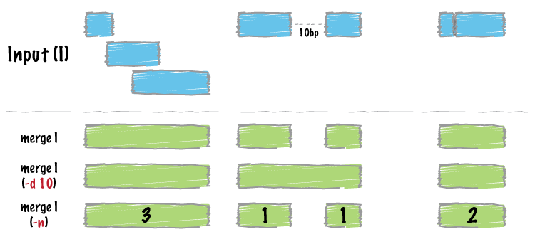
Many datasets of genomic features have many individual features that overlap one another (e.g. aligments from a ChiP seq experiment). It is often useful to just cobine the overlapping into a single, contiguous interval. The bedtools merge command will do this for you.

Input must be sorted

The merge tool requires that the input file is sorted by chromosome, then by start position. This allows the merging algorithm to work very quickly without requiring any RAM.

If your files are unsorted, the merge tool will raise an error. To correct this, you need to sort your BED using the UNIX sort utility. For example:

sort -k1,1 -k2,2n foo.bed > foo.sort.bed

Merge intervals.

Merging results in a new set of intervals representing the merged set of intervals in the input. That is, if a base pair in the genome is covered by 10 features, it will now only be represented once in the output file.

bedtools merge -i exons.bed | head -n 20
chr1    11873   12227
chr1    12612   12721
chr1    13220   14829
chr1    14969   15038
chr1    15795   15947
chr1    16606   16765
chr1    16857   17055
chr1    17232   17368
chr1    17605   17742
chr1    17914   18061
chr1    18267   18366
chr1    24737   24891
chr1    29320   29370
chr1    34610   35174
chr1    35276   35481
chr1    35720   36081
chr1    69090   70008
chr1    134772  139696
chr1    139789  139847
chr1    140074  140566

Count the number of overlapping intervals.

A more sophisticated approach would be to not only merge overlapping intervals, but also report the number of intervals that were integrated into the new, merged interval. One does this with the -c and -o options. The -c option allows one to specify a column or columns in the input that you wish to summarize. The -o option defines the operation(s) that you wish to apply to each column listed for the -c option. For example, to count the number of overlapping intervals that led to each of the new “merged” intervals, one will “count” the first column (though the second, third, fourth, etc. would work just fine as well).

bedtools merge -i exons.bed -c 1 -o count | head -n 20
chr1    11873   12227   1
chr1    12612   12721   1
chr1    13220   14829   2
chr1    14969   15038   1
chr1    15795   15947   1
chr1    16606   16765   1
chr1    16857   17055   1
chr1    17232   17368   1
chr1    17605   17742   1
chr1    17914   18061   1
chr1    18267   18366   1
chr1    24737   24891   1
chr1    29320   29370   1
chr1    34610   35174   2
chr1    35276   35481   2
chr1    35720   36081   2
chr1    69090   70008   1
chr1    134772  139696  1
chr1    139789  139847  1
chr1    140074  140566  1

Merging features that are close to one another.

With the -d (distance) option, one can also merge intervals that do not overlap, yet are close to one another. For example, to merge features that are no more than 1000bp apart, one would run:

bedtools merge -i exons.bed -d 1000 -c 1 -o count | head -20
chr1    11873   18366   12
chr1    24737   24891   1
chr1    29320   29370   1
chr1    34610   36081   6
chr1    69090   70008   1
chr1    134772  140566  3
chr1    323891  328581  10
chr1    367658  368597  3
chr1    621095  622034  3
chr1    661138  665731  3
chr1    700244  700627  1
chr1    701708  701767  1
chr1    703927  705092  2
chr1    708355  708487  1
chr1    709550  709660  1
chr1    713663  714068  1
chr1    752750  755214  2
chr1    761585  763229  10
chr1    764382  764484  9
chr1    776579  778984  1

Listing the name of each of the exons that were merged.

Many times you want to keep track of the details of exactly which intervals were merged. One way to do this is to create a list of the names of each feature. We can do with with the collapse operation available via the -o argument. The name of the exon is in the fourth column, so we ask merge to create a list of the exon names with -c 4 -o collapse:

bedtools merge -i exons.bed -d 90 -c 1,4 -o count,collapse | head -20
chr1    11873   12227   1   NR_046018_exon_0_0_chr1_11874_f
chr1    12612   12721   1   NR_046018_exon_1_0_chr1_12613_f
chr1    13220   14829   2   NR_046018_exon_2_0_chr1_13221_f,NR_024540_exon_0_0_chr1_14362_r
chr1    14969   15038   1   NR_024540_exon_1_0_chr1_14970_r
chr1    15795   15947   1   NR_024540_exon_2_0_chr1_15796_r
chr1    16606   16765   1   NR_024540_exon_3_0_chr1_16607_r
chr1    16857   17055   1   NR_024540_exon_4_0_chr1_16858_r
chr1    17232   17368   1   NR_024540_exon_5_0_chr1_17233_r
chr1    17605   17742   1   NR_024540_exon_6_0_chr1_17606_r
chr1    17914   18061   1   NR_024540_exon_7_0_chr1_17915_r
chr1    18267   18366   1   NR_024540_exon_8_0_chr1_18268_r
chr1    24737   24891   1   NR_024540_exon_9_0_chr1_24738_r
chr1    29320   29370   1   NR_024540_exon_10_0_chr1_29321_r
chr1    34610   35174   2   NR_026818_exon_0_0_chr1_34611_r,NR_026820_exon_0_0_chr1_34611_r
chr1    35276   35481   2   NR_026818_exon_1_0_chr1_35277_r,NR_026820_exon_1_0_chr1_35277_r
chr1    35720   36081   2   NR_026818_exon_2_0_chr1_35721_r,NR_026820_exon_2_0_chr1_35721_r
chr1    69090   70008   1   NM_001005484_exon_0_0_chr1_69091_f
chr1    134772  139696  1   NR_039983_exon_0_0_chr1_134773_r
chr1    139789  139847  1   NR_039983_exon_1_0_chr1_139790_r
chr1    140074  140566  1   NR_039983_exon_2_0_chr1_140075_r

bedtools “complement”

We often want to know which intervals of the genome are NOT “covered” by intervals in a given feature file. For example, if you have a set of ChIP-seq peaks, you may also want to know which regions of the genome are not bound by the factor you assayed. The complement addresses this task.

As an example, let’s find all of the non-exonic (i.e., intronic or intergenic) regions of the genome. Note, to do this you need a “genome” file, which tells bedtools the length of each chromosome in your file. Consider why the tool would need this information…

bedtools complement -i exons.bed -g genome.txt \
> non-exonic.bed
head non-exonic.bed
chr1    0   11873
chr1    12227   12612
chr1    12721   13220
chr1    14829   14969
chr1    15038   15795
chr1    15947   16606
chr1    16765   16857
chr1    17055   17232
chr1    17368   17605
chr1    17742   17914

bedtools “genomecov”

For many analyses, one wants to measure the genome wide coverage of a feature file. For example, we often want to know what fraction of the genome is covered by 1 feature, 2 features, 3 features, etc. This is frequently crucial when assessing the “uniformity” of coverage from whole-genome sequencing. This is done with the versatile genomecov tool.

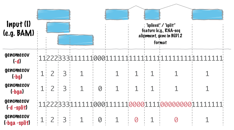
As an example, let’s produce a histogram of coverage of the exons throughout the genome. Like the merge tool, genomecov requires pre-sorted data. It also needs a genome file as above.

bedtools genomecov -i exons.bed -g genome.txt

This should run for 3 minutes or so. At the end of your output, you should see something like:

genome  0   3062406951  3137161264  0.976171
genome  1   44120515    3137161264  0.0140638
genome  2   15076446    3137161264  0.00480576
genome  3   7294047 3137161264  0.00232505
genome  4   3650324 3137161264  0.00116358
genome  5   1926397 3137161264  0.000614057
genome  6   1182623 3137161264  0.000376972
genome  7   574102  3137161264  0.000183
genome  8   353352  3137161264  0.000112634
genome  9   152653  3137161264  4.86596e-05
genome  10  113362  3137161264  3.61352e-05
genome  11  57361   3137161264  1.82844e-05
genome  12  52000   3137161264  1.65755e-05
genome  13  55368   3137161264  1.76491e-05
genome  14  19218   3137161264  6.12592e-06
genome  15  19369   3137161264  6.17405e-06
genome  16  26651   3137161264  8.49526e-06
genome  17  9942    3137161264  3.16911e-06
genome  18  13442   3137161264  4.28477e-06
genome  19  1030    3137161264  3.28322e-07
genome  20  6329    3137161264  2.01743e-06
...

Producing BEDGRAPH output

Using the -bg option, one can also produce BEDGRAPH output which represents the “depth” fo feature coverage for each base pair in the genome:

bedtools genomecov -i exons.bed -g genome.txt -bg | head -20
chr1    11873   12227   1
chr1    12612   12721   1
chr1    13220   14361   1
chr1    14361   14409   2
chr1    14409   14829   1
chr1    14969   15038   1
chr1    15795   15947   1
chr1    16606   16765   1
chr1    16857   17055   1
chr1    17232   17368   1
chr1    17605   17742   1
chr1    17914   18061   1
chr1    18267   18366   1
chr1    24737   24891   1
chr1    29320   29370   1
chr1    34610   35174   2
chr1    35276   35481   2
chr1    35720   36081   2
chr1    69090   70008   1
chr1    134772  139696  1

Sophistication through chaining multiple bedtools

Analytical power in bedtools comes from the ability to “chain” together multiple tools in order to construct rather sophisicated analyses with very little programming - you just need genome arithmetic! Have a look at the examples here.

Here are a few more examples.

1. Identify the portions of intended capture intervals that did not have any coverage:

@brent_p bedtools genomecov -ibam aln.bam -bga 
 | awk ‘$4==0’ | | bedtools intersect -a regions -b - > foo

— Aaron Quinlan (@aaronquinlan) January 10, 2014

2. Assessing the breadth and depth coverage of sequencing coverage in exome studies.

Principal component analysis

We will use the bedtools implementation of a Jaccard statistic to meaure the similarity of two datasets. Briefly, the Jaccard statistic measures the ratio of the number of intersecting base pairs to the total number of base pairs in the two sets. As such, the score ranges from 0.0 to 1. 0; lower values reflect lower similarity, whereas higher values reflect higher similarity.

Let’s walk through an example: we would expect the Dnase hypersensivity sites to be rather similar between two samples of the same fetal tissue type. Let’s test:

bedtools jaccard \
    -a fHeart-DS16621.hotspot.twopass.fdr0.05.merge.bed \
    -b fHeart-DS15839.hotspot.twopass.fdr0.05.merge.bed
intersection    union-intersection  jaccard n_intersections
81269248    160493950   0.50637 130852

But what about the similarity of two different tissue types?

bedtools jaccard \
    -a fHeart-DS16621.hotspot.twopass.fdr0.05.merge.bed \
    -b fSkin_fibro_bicep_R-DS19745.hg19.hotspot.twopass.fdr0.05.merge.bed
intersection    union-intersection  jaccard n_intersections
28076951    164197278   0.170995    73261

Hopefully this demonstrates how the Jaccard statistic can be used as a simple statistic to reduce the dimensionality of the comparison between two large (e.g., often containing thousands or millions of intervals) feature sets.

A Jaccard statistic for all 400 pairwise comparisons.

We are going to take this a bit further and use the Jaccard statistic to measure the similarity of all 20 tissue samples against all other 20 samples. Once we have a 20x20 matrix of similarities, we can use dimensionality reduction techniques such as hierarchical clustering or principal component analysis to detect higher order similarities among all of the datasets.

We will use GNU parallel to compute a Jaccard statistic for the 400 (20*20) pairwise comparisons among the fetal tissue samples.

But first, we need to install GNU parallel.

brew install parallel

Next, we need to install a tiny script I wrote for this analysis.

curl -O https://bedtools-tutorials.s3.amazonaws.com/web/make-matrix.py

Now, we can use parallel to, you guessed it, compute the 400 pairwise Jaccard statistics in parallel using as many processors as you have available.

parallel "bedtools jaccard -a {1} -b {2} \
         | awk 'NR>1' \
         | cut -f 3 \
         > {1}.{2}.jaccard" \
         ::: *.merge.bed ::: *.merge.bed

This command will create a single file containing the pairwise Jaccard measurements from all 400 tests.

find . \
    | grep jaccard \
    | xargs grep "" \
    | sed -e s"/\.\///" \
    | perl -pi -e "s/.bed./.bed\t/" \
    | perl -pi -e "s/.jaccard:/\t/" \
    > pairwise.dnase.txt

A bit of cleanup to use more intelligible names for each of the samples.

cat pairwise.dnase.txt \
| sed -e 's/.hotspot.twopass.fdr0.05.merge.bed//g' \
| sed -e 's/.hg19//g' \
> pairwise.dnase.shortnames.txt

Now let’s make a 20x20 matrix of the Jaccard statistic. This will allow the data to play nicely with R.

awk 'NF==3' pairwise.dnase.shortnames.txt \
| awk '$1 ~ /^f/ && $2 ~ /^f/' \
| python make-matrix.py \
> dnase.shortnames.distance.matrix

Let’s also make a file of labels for each dataset so that we can label each dataset in our R plot.

cut -f 1 dnase.shortnames.distance.matrix | cut -f 1 -d "-" | cut -f 1 -d "_" > labels.txt

Now start up R.

R

NOTE: The following example assumes that you have both the ggplot2 and RColorBrewer packages installed on your computer. If they are not installed, run both install.packages("ggplot2") and install.packages("RColorBrewer") from the R prompt and respond to the prompts that will follow.-

You should see something very similar to this:

R version 2.15.1 (2012-06-22) -- "Roasted Marshmallows"
Copyright (C) 2012 The R Foundation for Statistical Computing
ISBN 3-900051-07-0
Platform: x86_64-apple-darwin12.0.0 (64-bit)

R is free software and comes with ABSOLUTELY NO WARRANTY.
You are welcome to redistribute it under certain conditions.
Type 'license()' or 'licence()' for distribution details.

  Natural language support but running in an English locale

R is a collaborative project with many contributors.
Type 'contributors()' for more information and
'citation()' on how to cite R or R packages in publications.

Type 'demo()' for some demos, 'help()' for on-line help, or
'help.start()' for an HTML browser interface to help.
Type 'q()' to quit R.

>

No paste these commands into the R console:

library(ggplot2)
library(RColorBrewer)
blues <- colorRampPalette(c('dark blue', 'light blue'))
greens <- colorRampPalette(c('dark green', 'light green'))
reds <- colorRampPalette(c('pink', 'dark red'))
 
setwd("~/Desktop/bedtools-demo")
x <- read.table('dnase.shortnames.distance.matrix')
labels <- read.table('labels.txt')
ngroups <- length(unique(labels))
pca <- princomp(x)
qplot(pca$scores[,1], pca$scores[,2], color=labels[,1],     geom="point", size=1) +
  scale_color_manual(values = c(blues(4), greens(5), reds(5))) 

You should see this:

Et voila.

Note that PCA was used in this case as a toy example of what PCA does for the CSHL Adv. Seq. course. Heatmaps are a more informative visualization in this case since Jaccard inherently returns a measure of distance.

So let’s make a heatmap for giggles.

NOTE: The following example assumes that you have both the gplots package installed on your computer. If it are not installed, run install.packages("gplots") from the R prompt and respond to the prompts that will follow.-

library(gplots)
# thanks for the fix, Stefanie Dukowic-Schulze
jaccard_table <- x
jaccard_matrix <- as.matrix(jaccard_table)
heatmap.2(jaccard_matrix, col = brewer.pal(9,"Blues"), margins = c(14, 14), density.info = "none", lhei=c(2, 8), trace= "none")

You should see this:

Puzzles to help teach you more bedtools.

1. Create a BED file representing all of the intervals in the genome that are NOT exonic and are not Promoters (based on the promoters in the hESC file).

2. What is the average distance from GWAS SNPs to the closest exon? (Hint - have a look at the closest tool.)

3. Count how many exons occur in each 500kb interval (“window”) in the human genome. (Hint - have a look at the makewindows tool.)

4. Are there any exons that are completely overlapped by an enhancer? If so, how many?

5. What fraction of the GWAS SNPs are exonic? Hint: should you worry about double counting?

6. What fraction of the GWAS SNPs are lie in either enhancers or promoters in the hESC data we have?

7. Create intervals representing the canonical 2bp splice sites on either side of each exon (don’t worry about excluding splice sites at the first or last exon). (Hint - have a look at the flank tool.)

8. What is the Jaccard statistic between CpG and hESC enhancers? Compare that to the Jaccard statistic between CpG and hESC promoters. Does the result make sense? (Hint - you will need grep).

9. What would you expect the Jaccard statistic to look like if promoters were randomly distributed throughout the genome? (Hint - you will need the shuffle tool.)

10. Which hESC ChromHMM state (e.g., 11_Weak_Txn, 10_Txn_Elongation) represents the most number of base pairs in the genome? (Hint: you will need to use awk or perl here, as well as the groupby tool.)

answers